CS224w HomeWork 2
本文旨在记录CS224w Machine Learning With Graphs 2019完成作业中遇到的问题和作业的结果。
我的github仓库 LINK。
本部分共包含:
- Node Classi cation: correlation with Collective Classification and message passing
- Node Embeddings with TransE: correlation with Graph Representation Learning
Part 1 Node Classification
Node Classi cation主要是使用Collective Classification的方法,其主要流程和组成部分如下图所示:

其中approximate inference的方法主要为(这三者sort by how advanced these methods are):
- Relational Classification
- Iterative Classification
- Belief Classification
这三种方法都是基于Markov Assumption,即:
the labely $Y_i$ of one node depends on the labels of its neighbors, which can be mathematically written as:
$$P(Y_i|i)=P(Y_i|N_i)$$
其中$N_i$为节点i的neighbors。
Relational Classification
非常简单的方法,只使用了label和网络拓扑结构的信息,没有使用每个节点的features。对于每个无label节点的预测只是简单的取一个邻居的label的平均。
使用下式的公式来预测无label的节点。
其缺点也很明显,即
- The convergence not guaranteed.
- Cannot use node feature information, only use the graph information.
这部分对应的作业也比较简单,即在给定的简单的图上实现这个算法。
简易的代码如下:
1 | import snap |
运行代码即可得到Q1.1的答案。
Belief Propagation
Belief Propagation is a dynamic programming approach to answering conditional probability queries in a graphical model. 本质上是模拟网络上信息的传递,根据相邻节点传递的信息来确定自己的状态。在迭代过程中,每个节点都会跟相邻节点通信,即传递信息。详细的公式和细节见slide。
答案:
Part 2 Node Embeddings with TransE
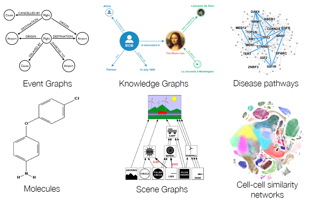
这里主要讨论一种经典的应用于Multi-relational graphs的embedding方法—-TransE。Multi-relational graphs是指:graphs with multiple types of edges. 这种图的一个典型例子就是知识图谱(Knowledge Graph)。而TransE也是知识图谱上面embedding的经典方法。
Part 3 GNN Expressiveness
NOTE:在进行训练的时候,如果节点没有features,其features vector设为全1向量或者该节点的度。
本部分主要在研究,GNN的层数与其表示能力(Expressiveness)的关系。expressiveness refers to the set of functions (usually the loss function for classi cation or regression tasks) a neural network is able to compute, which depends on the structural properties of a neural network architecture.
3.1 Effect of Depth on Expressiveness
3.2 Relation to Random Walk
3.3 Over-Smoothing Effect
3.4 Learning BFS with GNN
很简单的average aggregation,这里就不再写出。